I have a new paper out! Here is the much less technical write-up.

The link to the paper is here for more details: https://arxiv.org/abs/2610.10693

One thing in theoretical physics is that we want to study science at the most fundamental level, i.e. at smaller and smaller scales. What if I tell you that you can study that by observing the universe, in a programme now coined as a “cosmological collider”?

The energy E of a photon is proportional to the frequency f - the higher the frequency, the higher the energy carried. One UV photon carries more energy than one infrared photon. However, frequency is inversely proportional to wavelength, so the smaller the wavelength, the higher the frequency of light, and the higher the energy carried by a photon. This illustrates a rule of thumb in theoretical physics - if you want to look at smaller scale physics, you need to look at physics at high energy scale.

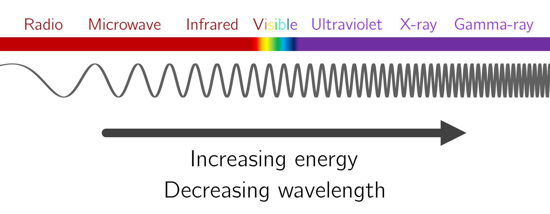
Smaller wavelength means higher energy.

This is why we build colliders like the Large Hadron Collider (LHC), and smash particles together at very high energies. However, in some sense, the energy scale in our particle colliders is still not that high - LHC "only" smashes protons at around 10^4 GeV. It turns out that if we are lucky, we might be able to get to 10^14 GeV by… just observing the universe!

This crazy idea was first proposed by two physicists Xingang Chen and Yi Wang in 2009 [1, 2], but they gave it a rather boring name “quasi-single field inflation”. Then in 2015, Juan Maldacena and Nima Arkani-Hamed systematically studied how to implement this idea and gave it a catchy name of “cosmological collider”[3], and it took off.

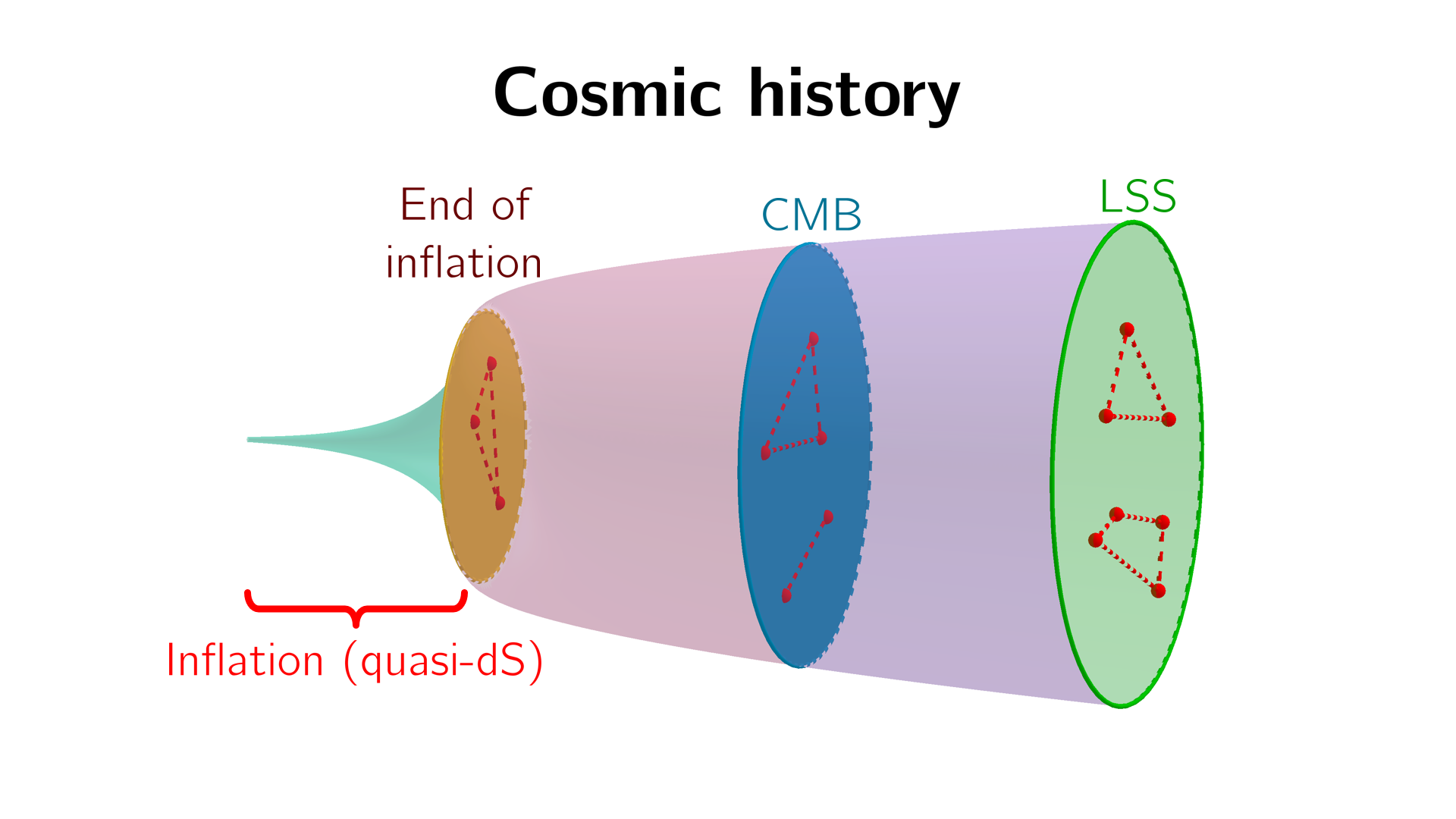
Illustration of the cosmic history in our leading model, starting with a period of exponential expansion known as cosmic inflation.

To explain the idea, we need to look at the current leading model of the cosmic history. In the first fractions of a second, there was a period of exponential expansion in the very beginning of the universe known as cosmic inflation, first proposed by Alan Guth [4]. Technically, we have not proved the existence of this cosmic era, but it solved so many problems in cosmology that it is widely accepted, though not without opponents. Here we assumed this did happen.

During inflation, the energy scale can be as high as 10^13 - 10^14 GeV [5], around 10 orders of magnitude higher than what can be achieved at the LHC (10^4 GeV). There should be high-energy processes happening during that time, and if there really were massive particles produced during that time, we want to detect them. However, unlike at the LHC, where we can smash particles at our will, we cannot go back to this period of inflation to actually do experiment and detect the particle right then and there. So what should we do?

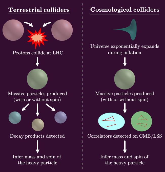
Comparison between “terrestrial colliders” like the LHC and a “cosmological collider”.

The answer is that if these massive particles decay into massless ones, it leaves behind a very distinct fingerprint that tells us their mass and their spins. And if we have a powerful enough telescope, and high enough computational power, we should be able to detect these signatures.

This is actually very similar, at least in spirit, to how we detect particles at the LHC. When we smash protons together, the high energies can potentially produce heavy particles, the most famous example of which is the Higgs boson. But we didn’t directly detect the Higgs boson; we detected its decay products. The fact that the Higgs boson existed affected the distribution of these decay products, and this is some sort of fingerprint which we can analyse and even deduce the mass and the spin of said particle. This is where the name “cosmological collider” comes from.

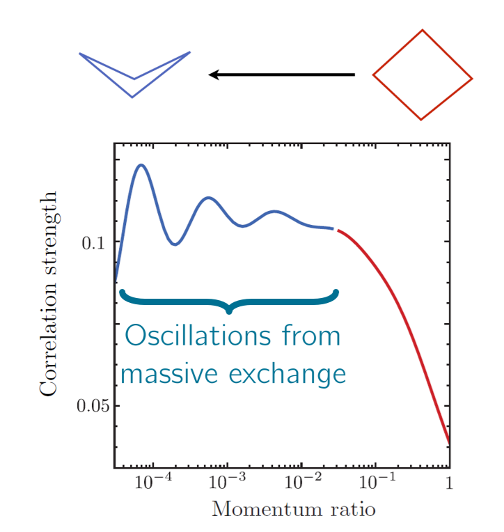
Illustration (not to scale) of the oscillatory signals in the so-called “collapsed limit of the trispectrum.”
Credit: Daniel Baumann’s lecture notes on cosmological correlators, accessible here.

But what are these fingerprints? They come in the form of oscillations, and in fact, the frequency of these oscillations is directly linked to the mass of these heavy particles. So far, the error bars have been comically bad: a particular measurement of the amplitude of one of these signals reads -0.9 ± 5.1 [6], and the best so far seems to be 467 ± 140 [7], both of which are consistent with 0, but we hope that this improves in the future.

As someone working on this, I think it’s only fair to also tell you the limitations to this “cosmological collider” programme. Assuming cosmic inflation really happened, did it really have that high energy of 10^13 - 10^14 GeV? If you dig into the maths, these heavy particles actually need to have mass roughly on par with the energy scale of inflation - any lighter will yield no oscillations, any heavier will make this oscillatory signal heavily suppressed, and we could not see them. That said, it is still a hopeful direction in search of new fundamental, high-energy physics.

So… what is our paper about?

In essence, we want to see, from a theoretical perspective, whether we can gain even more information than just mass and spin of the particle, if we were really able to see these oscillations. Our approach is to start from the ground up: first find out what properties a particle can theoretically have during inflation, then ask whether all these properties can be observed now.

It turns out that there is a limited number of properties a particle can have during inflation. In other words, not every single theory of particles during inflation can meet the “minimum requirement” of being physically plausible. Here are the “minimum requirements”:

1) Spatial rotational invariance (also known as SO(3))

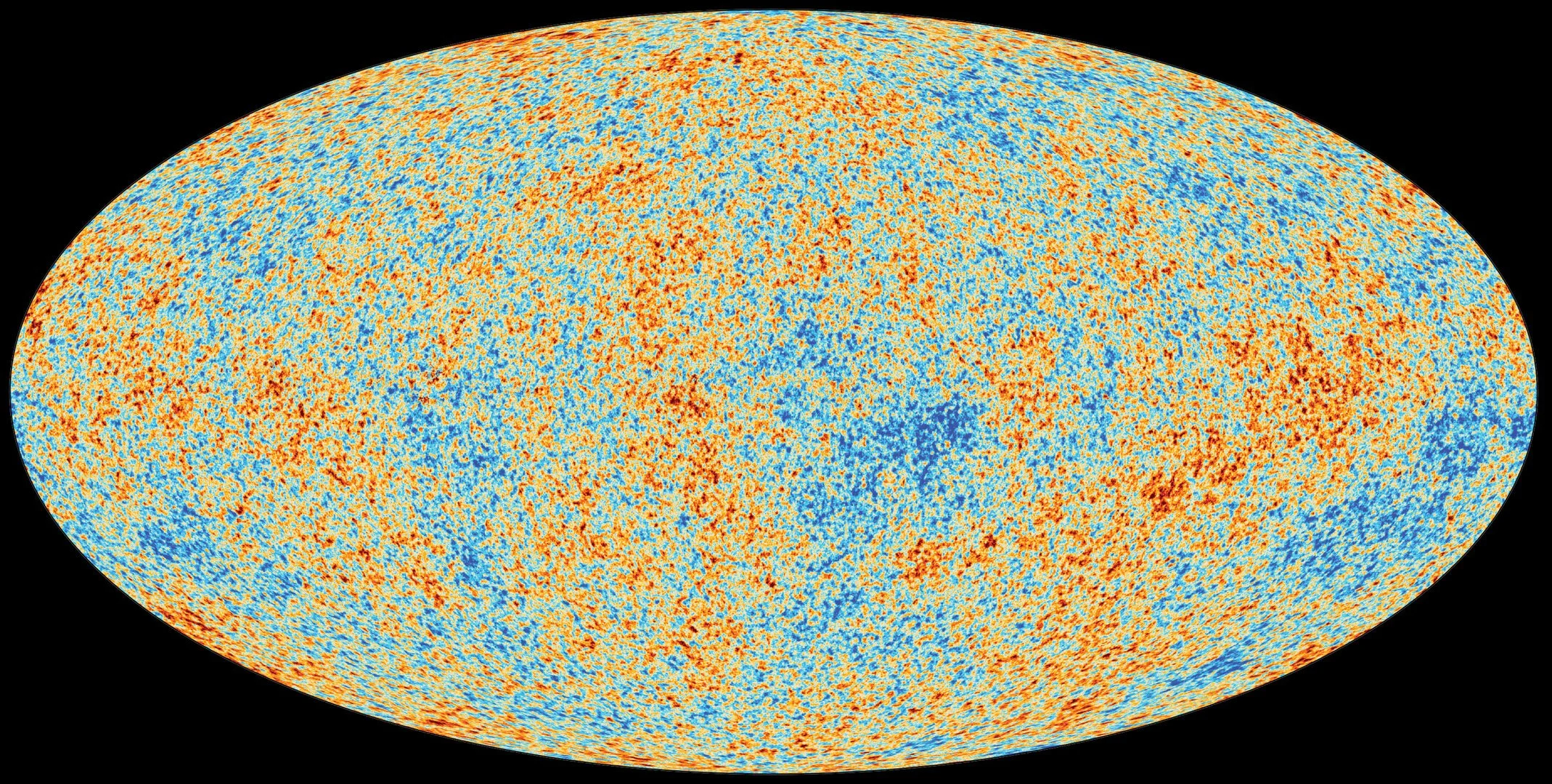
The Cosmic Microwave Background (CMB). Each dot represents the temperature of the photons emitted from roughly 380000 years after the Big Bang, red means hotter, blue means colder. Differences between the hot spots and cold spots are exaggerated by 10^5 times. These fluctuations in temperature are roughly the same in every direction. Credit: ESA

To a good degree of approximation, the universe is spatially isotropic - the same in every direction. It does not matter which direction you point your telescopes in; statistically speaking, the distribution looks roughly the same. We want this rotational symmetry to manifest itself for these heavy particles too. In the framework of quantum field theory (QFT), each particle is an excitation of the underlying quantum fluctuations, and we want these fluctuations to be the same in every direction.

2) Bunch-Davies vacuum conditions

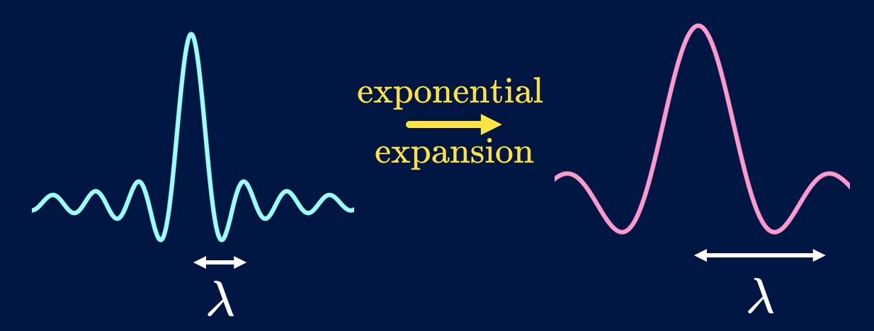
Waves stretch exponentially with the universe. So the rate of expansion was slower in the far past, to the point where these waves behave as if the universe did not expand.

This one is a bit technical, but here is the gist: waves / fluctuations stretch together with the universe, in fact stretching exponentially fast. If we dial the clock back, the rate of stretching was very slow in the far past, to the point that the waves don’t really “feel” the expansion of the universe. So our theory of the heavy particles during inflation needs to allow them to not feel the expansion in the far past.
3) Microcausality (information cannot travel faster than light)

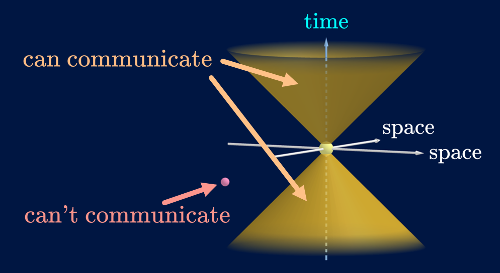
The yellow dot in the middle can communicate with anyone inside the double-cone, because that only requires slower-than-light communication. However, the yellow dot in the middle can’t communicate with the pink dot on the left, because that requires faster-than-light communication.

This condition simply boils down to “information cannot travel faster than the speed of light”. By digging into the maths, this condition turns out to link to complex analysis, and is surprisingly restrictive. In fact, this idea of causality being surprisingly restrictive has been observed not just in cosmology, but also in particle physics (see, e.g. [8]) decades ago.

There is another technical requirement known as scale invariance. This is a symmetry that the universe has been observed to have, and is in fact a strong evidence for the period of inflation to have existed. In this work, we only considered one particular type of particle (or field in the language of QFT) known as a vector boson / field, but this focus is mainly because of simpler calculations. The analysis does not fundamentally change when we consider other types of particles, other than being computationally more difficult.

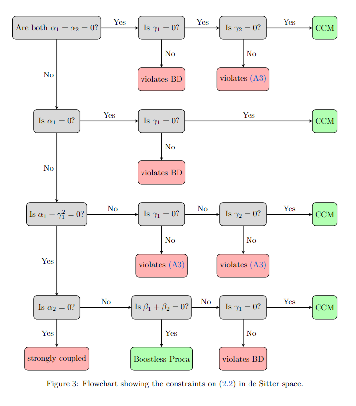
The flowchart describing the procedure we use: depending on the different scenarios, we check against these “minimum requirements”. The green boxes show that those theories pass through the minimum requirements, while the red ones show they violated at least 1 of the requirements. Taken from our paper.

At the end, our analysis shows that there are 5 properties such a vector boson can have, and in principle, all these 5 properties can be observed, if we have a powerful enough telescope, and better data analysis techniques to decode these oscillations.

Overall, the project seems like we are playing little games - look at the flowchart above: we simply need to check in each theory whether they satisfy those minimum requirement. If they don’t, we can discard them straight away. There are definitely straightforward generalisations of our project available, e.g. what about tensor bosons? But for a moment, I am working on proving a little observation (and calculation trick) I had during this project, and it’s looking quite promising. Of course, I don’t want to spill the beans just yet… watch this space (pun intended)!